59 Model Selection and Checking
59.1 Introduction
In this section we’ll explore the types of models that are used in time-series analysis. As you read, try to develop a general understanding of the concepts, some of which we’ll apply as part of this week’s practical session.
59.2 What are time-series models?
Time-series models are a ‘class’ of statistical models specifically designed for analysing data that is recorded sequentially over time.
As we’ve learned, they’re used to:
- understand underlying patterns in the data, such as ‘trends’, ‘seasonality’, and ‘cycles’.
- make predictions about future values based on observed historical data.
Various types of time-series models can be used depending on the specific characteristics of our data and the objectives of our analysis. Some common types include:
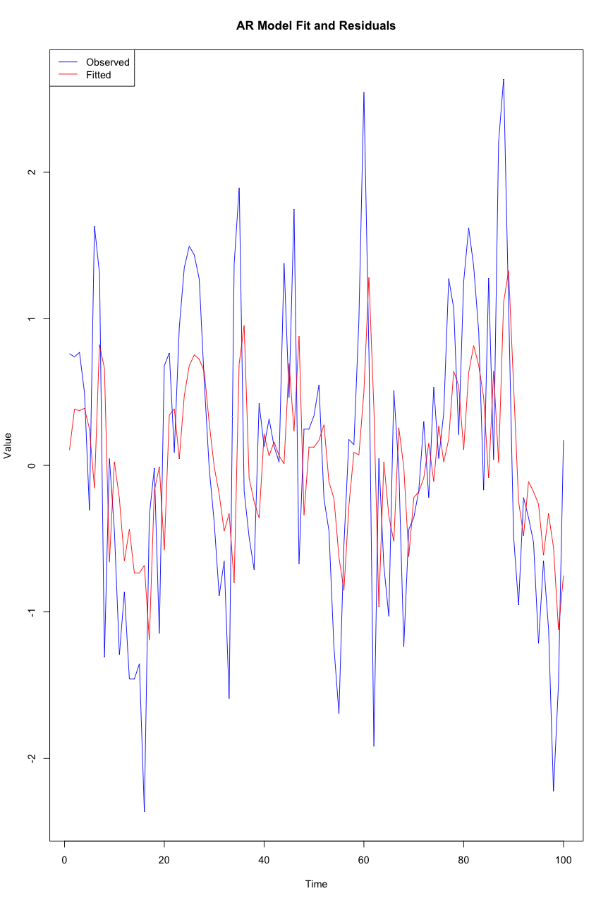
Autoregressive (AR) models
‘Autoregressive’ models predict future values based on past values of the same variable. An AR model uses the dependence between an observation and a number of lagged observations.
Unlike some other models, AR models rely solely on their own previous values for forecasts. For example, we might predict an athlete’s performance tomorrow based on their performance over the last few days.
Moving Average (MA) models
‘Moving average’ models use the dependency between an observation and a residual error from a moving average model applied to lagged observations. They focus on the noise or error of past observations.
Like AR models, MA models depend only on past data for forecasting. However, MA models focus on the error component of past predictions rather than the values themselves. For instance, adjusting future game strategy based on the error in predicted vs. actual outcomes of past games.
Autoregressive Moving Average (ARMA) models
ARMA models combine AR and MA models, using both past values and past forecast errors to predict future values. This hybrid approach can capture more complex patterns.
ARMA models are more versatile for more complex time-series which neither AR nor MA could model efficiently alone. For example, we might want to analyse and forecast a player’s performance trends over a season, taking into account both their performance and deviations from expected outcomes.
Autoregressive Integrated Moving Average (ARIMA) models
ARIMA models are an extension of ARMA models that also include differencing of observations to make a non-stationary time series stationary. This process allows them to handle data with trends over time.
ARIMA extends ARMA models by incorporating differencing, making it suitable for data with trends and seasonality, like predicting seasonal ticket sales for sports events. You’ll recall that we previously treated differencing as a separate stage of analysis, but ARIMA incorporates this into one procedure.
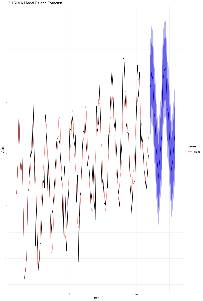
Seasonal Autoregressive Integrated Moving-Average (SARIMA) models
SARIMA models extend ARIMA models by specifically addressing and modeling seasonality in data, allowing for more accurate forecasts in data with strong seasonal patterns.
This type of model builds on ARIMA by adding seasonality components, making it highly effective for forecasting where data shows clear seasonal trends, such as predicting peaks in athlete performance during certain times of the year.
Vector Autoregression (VAR) models
VAR models are used to capture the linear interdependencies among multiple time-series. Each variable in a VAR is modeled as a linear function of past values of itself and past values of all other variables in the system.
Unlike the previous univariate models (AR, MA, ARMA, ARIMA, SARIMA), VAR models are multivariate and can analyse and forecast multiple time-series simultaneously (like examining the relationship between team performance, ticket sales, and merchandise sales).
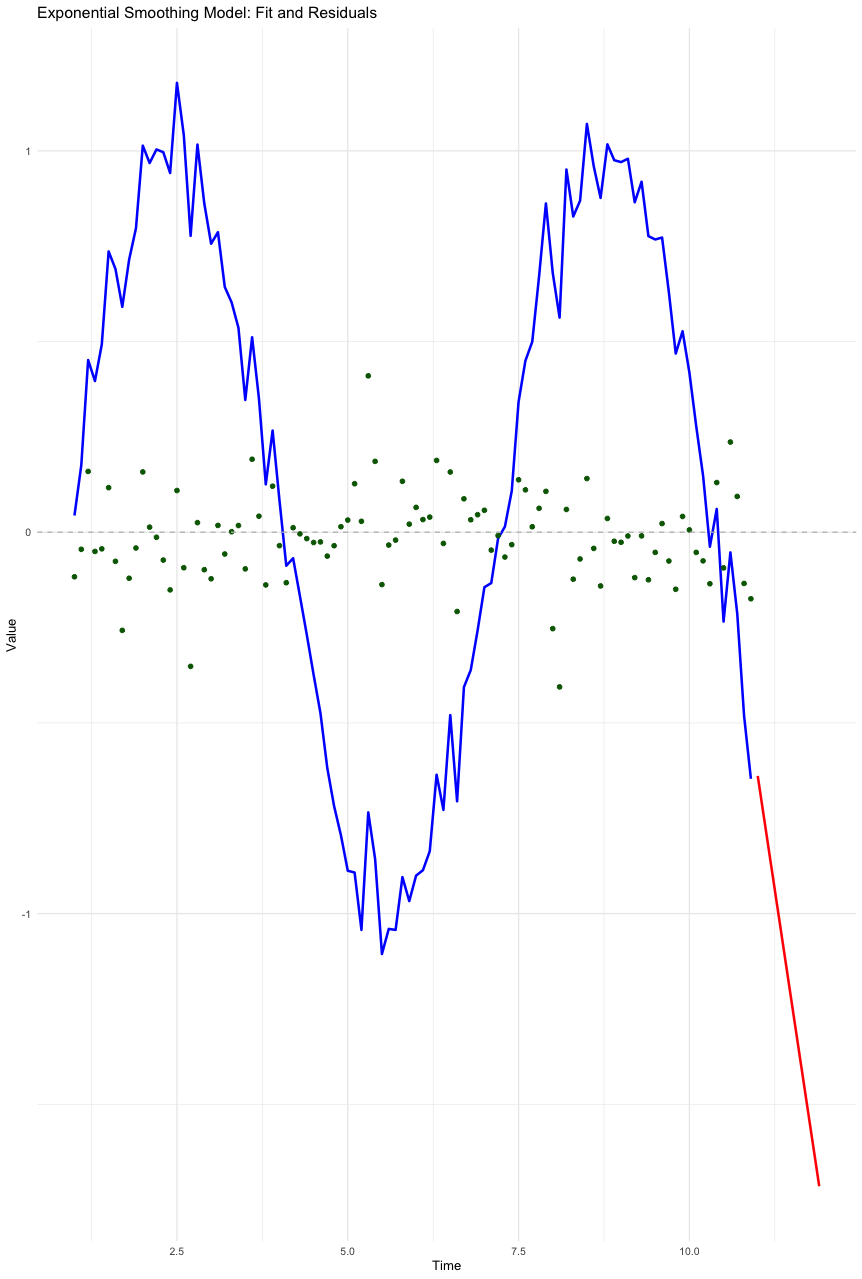
Exponential Smoothing (ES) models
Exponential Smoothing models are forecasting methods that apply smoothing factors to make forecasts. These models can easily adjust to data trends and seasonal patterns by applying more weight to more recent observations.
ES models differ from the others by emphasising recent observations more heavily. This makes them very suitable for data with non-linear patterns, like forecasting sudden changes in player performance due to injuries or unexpected events. Often, it makes sense to assume that things we have observed more recently are likely to have greater predictive power than things we observed in the past. Unlike ARIMA or SARIMA, ES models are better at handling changing trends and seasonality with simpler parameters.
59.3 How do we choose which model to use?
In practical applications, the choice of a time series model depends on:
the specific characteristics of your data;
the theoretical understanding of the underlying processes, and;
the forecasting or explanatory needs of the analysis you’re conducting.
From the previous summary of the seven main types of TSA model, you should have a good idea of when each of the models might be more (or less) useful.
In addition to this, there are statistical tools available that allow us to evaluate the effectiveness of the models that we choose.
This is called ‘criterion-based selection’.
The concepts here are similar to those we encountered in some of the other model-building techniques covered earlier in the module, such as Path Analysis.
Criterion-Based Selection
Criterion-based selection methods provide quantitative measures to compare and evaluate the performance of different time-series models.
By applying these criteria to our models, we can choose a model that not only fits the historical data well but also balances the complexity of the model with its predictive power.
This balance is crucial in avoiding overfitting, where a model captures the noise instead of the underlying pattern in the data, and underfitting, where the model is too simplistic to capture the data’s dynamics.
Overfitting and underfitting are two common issues faced during the model building process:
‘Overfitting’ occurs when a model learns the detail and noise in the training data to the extent that it performs well on the training data, but doesn’t generalise well to new, unseen data. Essentially, the model becomes too complex. As a result, it may show high accuracy on training data but performs poorly on validation or test data, making it pretty useless.
‘Underfitting’ happens when a model is too simple to detect the underlying patterns in the data, and fails to achieve a good performance on both the training data and testing data. The model doesn’t have enough complexity or it’s not trained sufficiently, leading to poor predictions.
Akaike Information Criterion (AIC)
The Akaike Information Criterion (AIC) is a common measure for model selection, particularly in time series analysis. We have already utilised it in previous sections of this module.
It’s based on the concept of information entropy, providing a relative estimate of the information lost when a given model is used to represent the process generating the data.
The AIC is calculated as:
\[ AIC = 2k - 2ln(L) \]
where \(k\) is the number of parameters in the model and \(L\) is the likelihood of the model.
The key aspect of AIC is its penalty for the number of parameters, which discourages overfitting.
In practical terms, when comparing multiple models, the one with the lowest AIC is generally preferred, as it suggests a better balance between goodness of fit and simplicity.
Bayesian Information Criterion (BIC)
Similar to AIC, the Bayesian Information Criterion (BIC) is another crucial tool for model selection.
Introduced by Gideon Schwarz, the BIC is also known as the Schwarz Information Criterion (SIC). It is calculated as:
\[ BIC=ln(n)k−2ln(L) \]
where \(n\) is the number of observations, \(k\) is the number of parameters, and \(L\) is the likelihood of the model.
The BIC places a higher penalty on the number of parameters than AIC, especially when the sample size is large.
This characteristic makes BIC more ‘strict’ against complex models, potentially favouring simpler models compared with the AIC.
In model comparison, the model with the lowest BIC is usually preferred (just like the AIC), indicating a better trade-off between model complexity and fit to the data.
Residual Diagnostics
AIC, BIC and Adjusted R-squared are examples of criterion-based methods of evaluating our model. They give us numbers to evaluate and compare.
Another technique is called ‘residual diagnostics’. Residuals (the differences between observed and predicted values) offer lots of information about a model’s performance.
By systematically examining the properties of these residuals - specifically their autocorrelation, homoscedasticity, and normality - we can evaluate the adequacy of our model and identify areas for improvement.
Autocorrelation in Residuals
Autocorrelation is the correlation of a time series with its own past and future values.
In the context of residuals, it’s important to check for autocorrelation because its presence indicates that the model has not fully captured the information in the data, particularly in the time domain.
To assess autocorrelation, we often use tools like the Durbin-Watson statistic or the Ljung-Box Q-test.
A lack of significant autocorrelation in the residuals suggests that the model has adequately accounted for the time-dependent structure in the data.
Homoscedasticity of Residuals
Homoscedasticity implies that the residuals have constant variance across time.
Heteroscedasticity, the opposite, suggests that the model’s error terms vary at different times, indicating that the model may not be equally effective across the entire dataset.
This can be particularly problematic in forecasting, as it implies changing uncertainty levels over time.
Techniques such as plotting residuals against time or fitted values, and conducting tests like the Breusch-Pagan or White’s test, are employed to detect homoscedasticity.
A model yielding homoscedastic residuals is generally preferred, as it indicates consistent performance across different time periods.
Normality of Residuals
As you know, the assumption of normality in residuals is central to many statistical inference techniques.
If the residuals are normally distributed, it suggests that the model has successfully captured the underlying data distribution, and the error term is purely random.
This can be assessed using graphical methods like Q-Q plots or more formal tests like the Shapiro-Wilk test.
Non-normal residuals might indicate model misspecification, outliers, or other issues that could affect the reliability of the model’s forecasts.
59.4 Model Checking
We’ve discussed how we can go about selecting which model to use, and how to compare the performance of one model against another. This can be helpful when we have different types of model that we want to create, and compare their performance.
Model checking develops this idea; it aims to evaluate how effective our model is.
Some of the concepts are similar to those discussed above.
Residual Analysis
Residual analysis is important in time-series model checking, especially for verifying that the residuals behave like white noise.
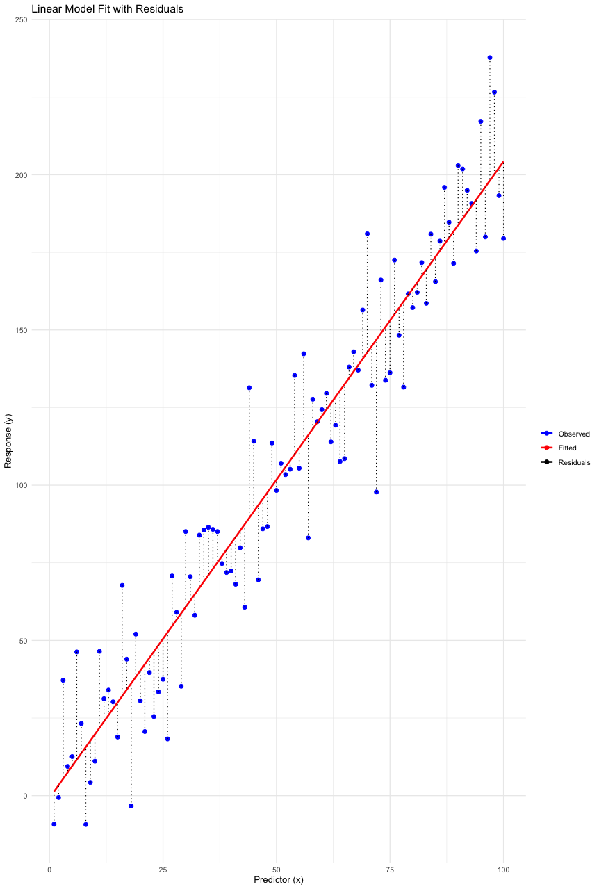
‘Model residuals’ are the differences between observed values and the values predicted by a model. For example, our model might predict that 520 people will attend a game. If 480 people actually attend, the residual is 40. In the context of statistical modeling and machine learning, residuals play a crucial role in diagnosing and improving model performance. Residuals are essentially the errors in predictions, offering insights into the accuracy and efficacy of a model.
White noise residuals indicate that the model has successfully captured the underlying structure of the time-series data. To assess if residuals are white noise, we should check for three key characteristics: lack of autocorrelation, zero mean, and constant variance.
The absence of autocorrelation can be verified using the Ljung-Box Q-test or by examining the autocorrelation function (ACF) plot, where no significant autocorrelations at various lags would suggest randomness.
The zero mean property can be checked using simple descriptive statistics, ensuring that the mean of the residuals is not significantly different from zero.
Constant variance, or homoscedasticity, in the residuals is another essential criterion. It ensures that the model’s predictive accuracy remains uniform across the entire time series.
To check for constant variance, visual inspection of residual plots against time or predicted values can be used. In these plots, residuals should display no discernible patterns or trends, and their spread should remain consistent across the range of values.
Formal statistical tests like the Breusch-Pagan or White’s test can also be used to statistically validate homoscedasticity. If the residuals exhibit white noise characteristics, it implies that the model has effectively captured the information in the time series, making it a suitable choice for forecasting.
Conversely, if these conditions are not met, it may indicate model inadequacies, necessitating further refinement or the selection of an alternative model.
Accuracy Metrics
Finally, in addition to the above, we can calculate some metrics that measure the accuracy of our model in terms of its predictive power:
Mean Absolute Error (MAE) is a straightforward metric used in evaluating the accuracy of a time series model.
It calculates the average magnitude of errors between the predicted and actual values, without considering their direction. The MAE is particularly useful in scenarios where all errors, regardless of their direction, are equally important.
ts simplicity and interpretability make it a popular choice for a primary assessment of model performance. However, it does not highlight larger errors, as it treats all deviations equally, potentially underestimating the impact of significant prediction errors.
Root Mean Squared Error (RMSE) is another critical metric for assessing the accuracy of time series models.
Unlike the MAE, RMSE penalises larger errors more severely by squaring the residuals before averaging and then taking the square root of the result. This characteristic makes RMSE sensitive to large errors, thus it is useful in applications where large deviations are particularly undesirable.
However, its sensitivity to outliers means that RMSE can give a distorted impression of model performance if the dataset contains significant anomalies or noise.
Mean Absolute Percentage Error (MAPE) offers a perspective on model accuracy in terms of percentage errors, making it a really intuitive measure for expressing the accuracy of our model in relative terms.
It calculates the average of the absolute percentage errors between the predicted and actual values. MAPE is especially useful when comparing the performance of models across different scales or datasets.
However, its reliance on percentage errors means it can be misleading in cases where the actual values are very low or zero, leading to undefined or infinite errors, and thus requires careful interpretation in such scenarios.